Introduction

McMaille (pronounce : MacMy) is a program for indexing powder patterns by Monte Carlo and grid search (maille in french = cell in english). The 2-theta peak positions extracted from a peak hunting program are used together with the intensities in order to build a pseudo powder pattern to which are compared patterns calculated from the cell parameters proposed by a Monte Carlo or by a grid systematic search process. In McMaille versions 0.9-2.0, the calculated intensities were adjusted by a Le Bail fit (applying 3 iterations of the Rietveld decomposition formula) using Gaussian peak shapes. In version 3.0, time is gained by a factor 20 by using columnar peak shapes and a "fit" by percentage of inclusion of the calculated columns inside the "observed" one. The best cells are refined, more or less. This is similar to the (unnamed and still unavailable ?) software by B.M. Kariuki et al., J. Synchrotron Rad. 6. (1999) 87-92, though the latter uses a genetic algorithm and the raw data. Moreover, McMaille proposes an option of simultaneous two phases indexing and an automated expert system (black box mode) with a simplified manual (recommended for beginners).

Version 4.00 is available under two executables, one for single processor machines and another one parallelized for multi core machines (core duo, dual core, quad core etc), much faster. 

Main improvements in version 4.00 :
- parallelization for core duo (=dual core), quad core multiprocessors,
- volumes examined in black box mode were enlarged,
- Bravais lattice identification,
- more help provided for the identification of the most plausible cells in the lists of possible hits (the most plausible cell is proposed at the bottom of the output file with .imp extension),
- more clarity with shorter lists of cells (cutted to the 20 best of them)
- new lists ordered by best figure of merit (FoM) F(20) and M(20) and by the Rp-based special McMaille FoM (McM20) taking account of the Bravais lattice and level of symmetry,
- old bugs corrected, like trapping in small volume regions taking excessive long time.

Armel Le Bail  -  Last update : November 2006

McMaille version 4.00 is distributed under the GNU Public Licence conditions. 

The zipped package contains the executable for Windows 95/98/NT/XP, as well as the FORTRAN source codes (quite short and documented) for both the single and the multi processor machines, and some examples described below. 

The compiler used for building the executable was Intel Visual Fortran 9.1. The parallelized version is realized by using OpenMP directives. 
 

The package MvMaille-V4.zip contains mainly :

  McMaille.exe      : executable for MS Windows, single processor
  McMaille.for       : the FORTRAN source code
  license.html         : the GNU Public License (GPL) 

  PMcMaille.zip     : contains the executable for the multi core processors 
                      (named McMaille.exe) and a DLL named libguide40.dll
                      which has to be installed in the same directory. The corresponding
                      source code McMaille.for with OpenMP directives is also there.

  McMaille-v4.html  : the complete manual
  short-manual.html : a short manual version for the automated "black-box mode

  McMaille.pdf        : copy of the McMaille publication
  benchmarks.pdf    : copy of the benchmarks publication

  tests.zip                : various classical test files
  benchmarks.zip    : more test files (benchmarks)
  sdpdrr2.zip           : more test files (from the 'Structure Determination
                                     by Powder Diffractometry Round Robin 2')

  cub.hkl, hex.hkl, rho.hkl, tet.hkl, ort.hkl, mon.hkl, tri.hkl
                               : the prepared lists of hkl Miller indices which have
                                        to be installed in the same directory as the McMaille.exe program 
 window.jpg           : figure called by the McMaille-v4.html file (the manual)
 McM-ico.ico         : icon file, if you wish to put it as a shortcut on the screen
 McM-large.gif      : same image as the icon above, slightly larger
 example.gif           : figure showing the display of a .prf file by WinPLOTR

More about the .hkl files :
You should absolutely let the cub.hkl, hex.hkl, rho.hkl, tet.hkl, ort.hkl, mon.hkl, tri.hkl files in the same directory as McMaille.exe as well as your parameters .dat files. These .hkl files contain a list of predetermined Miller indices ordered according to a cell having a, b, c, parameters close to each other. 

In case of successful use, please cite the paper :
 A. Le Bail, Powder Diffraction 19 (2004) 249-254.
                                      (included into the package)

See comparisons of indexing software including McMaille :
J. Bergmann, A. Le Bail, R. Shirley and V. Zlokazov,  Z. Kristallogr. 219 (2004) 783-790.
                                      (included into the package)

Visit the Indexing Benchmarks Web page at :
               http://www.cristal.org/uppw/benchmarks/

The manual : McMaille-v4.html included in the package is also available at :
              http://www.cristal.org/mcmaille/
         or at http://www.cristal.org/mcmaille/

Read the paper cited above for full details.

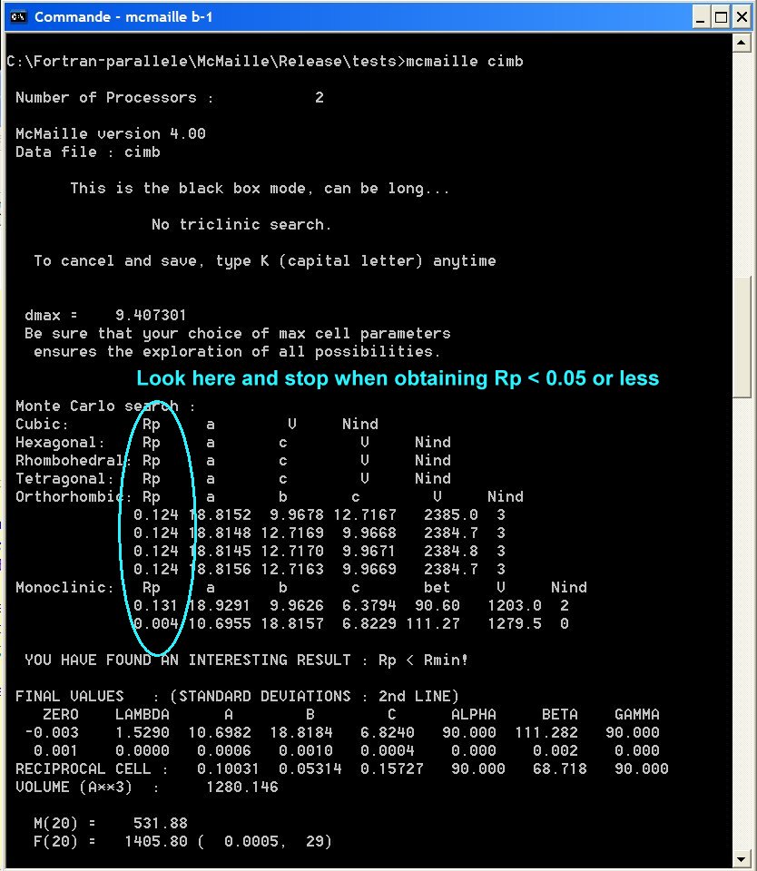
As soon as a Monte Carlo cell proposal produces Rp < Rmaxref ~0.5 (similar definition as Rp in the Rietveld method), that cell is more closely examined. Because a least square refinement would not be efficient, the cell parameters are changed (NCYCLES times, see below) a bit (in the range 0. to 0.02 Angstroms and 0. to 0.2 degrees), randomly by using the Monte Carlo process, around their initial values, checking if Rp decreases. Most of the times Rp decreases enormously, sometimes below the selected Rmax (a limit value for keeping the cell) and Rmin (another limit value for stopping the run because, with such a fit quality,  the cell could be the right one). This cell adjustment is analogous to simulated annealing. Moreover, a second criterium is used being that if the number of expected peaks is explained (NDAT-NIND) with Rp > Rmaxref, that proposal cell is examined too. This is a brute force indexing approach, very simple to develop. Least square parameters refinements (using the old CELREF routine by Laugier & Filhol) are performed at the end on the selected cell(s). 

Some important values defined in the program are below : 

               Nhkl Min   Nhkl Max   NCYCLES    NTRIED/NSOL
cubic            6xNDAT     400       200          100
rhombohedral    12xNDAT     600       500         1000
hexagonal       12xNDAT     800       500         1000
tetragonal      12xNDAT     800       500         1000
orthorhombic    20xNDAT    1000      1000        10000
monoclinic      20xNDAT    1000      2000       100000
triclinic       20xNDAT    1000      5000       100000

NDAT    = Number of powder pattern peaks examined
Nhkl    = Number of calculated hkl compared to the data
           (read in the .hkl files)
NCYCLES = Number of random parameter small changes for a given
          selected cell proposal (having Rp < Rmaxref)
NTRIED  = Number of Monte Carlo events
NSOL    = Number of solutions retained having Rp < Rmax
       
The NTRIED/NSOL ratio helps to reduce the number of retained
cells. If the value is < to the numbers listed above, then
Rmax is decreased by 5%. However, the process is not active
if NSOL < 50 and Rmax should be given negative. Avoiding being
overloaded by cell proposal is better resolved by decreasing
the control parameters W (peak width) and/or Nind (number of
non-indexed peak positions tolerated) and/or Rmaxref (the Rp
level below which a cell will be refined).

The figures of merit (F.o.M.) as applied in McMaille

There are 4 F.o.M. used in McMaille :

1 - Classical P.M. de Wolff (1968):  M20
    P.M. de Wolf, J. Appl. Cryst. 1 (1968) 108-113.

2 - Classical Smith & Snyder (1979): FN (F20 for N=20)
    G.S. Smith and R.L. Snyder, J. Appl. Cryst. 12 (1979) 60-65.

3 - Rp which is equivalent to a Rietveld profile R factor.
    H.M. Rietveld, J. Appl. Cryst. 2 (1969) 65-71.

4 - The Rp-based new McMaille F.o.M. McM20 is calculated, for 20 
    observed lines, as :

     McM20 = [100./(Rp*N20)] * Brav * Sym

where :
  N20 is the number of possibly existing lines up to the 20th 
      observed line (for a P lattice).
  Brav is a factor equal to 6 for F and R Bravais lattices, 4 for I,
      2 for A, B, C and 1 for P.
  Sym is a factor equal to 6 for a cubic or a rhombohedral cell,
      4 for a trigonal/hexagonal/tetragonal cell, 2 for an 
      orthorhombic cell, and 1 for a monoclinic or triclinic cell.

Note that the M(20) and F(20) above are proposed without taking 
account of extinctions (P lattice).

The larger are M20, F20 and McM20, and the better the solution. For
Rp, this is the reverse, the more Rp is small, and the better is the
fit. 

McM20 is the best at separating clearly the most probable solutions
due to the consideration of symmetry and Bravais lattices.

However, F20 and M20 may be artificially high in McMaille because some
lines can be eliminated at the refinement stage if they show
excessive discrepancy (decreasing the average discrepancy...). 

Running McMaille (by either clicking on McMaille.exe and giving the entry file name - no extension - or in a DOS box by typing "McMaille name" ) requires a parameters data file. A typical data file (should be named name.dat, name being your choice) follows : 

Sr2Cr2O7                       Title
1.54056 0.0 2                  Wavelength, Zeropoint, Ngrid
1 1 1 0 0 0                    Symmetry codes
0.16 6                         W , Nind
3. 15. 200. 1500. 0.1  0.2 0.4 Pmin, Pmax, Vmin, Vmax, Rmin, Rmax, Rmaxref
0.2 0.2                        Spar, Sang  (grid search only)
20000  1                       Ntests, Nruns (Monte Carlo only)
!!!                        A line starting by ! is ignored
11.180   345.                  2-theta (or d(A)), Intensity
12.217  1120.                  Etc
15.835   124.                  20 couples of positions and
18.709   455.                     intensities should cover usual
Etc                               cases, but more may be 
                                  necessary (max = 100)
Or, if W above is negative :
11.180   345.   0.16          2-theta, Intensity, W
12.217  1120.   0.10          Etc
15.835   124.   0.24          triplets of positions,
18.709   455.   0.16              intensities and widths
Etc              

In Black box mode, the file is much shorter :

Sr2Cr2O7                       Title
1.54056 0.0 -3                  Wavelength, Zeropoint, Ngrid
!!!                        A line starting by ! is ignored
11.180   345.                  2-theta, Intensity
12.217  1120.                  Etc
15.835   124.                  20 couples of positions and
18.709   455.                     intensities. You may put more
Etc                               but only 20 will be used.          

Wavelength : your experiment wavelength. If you used CuKalpha, you should have stripped alpha2 before peak positions hunting. If you try to index large cells (proteins, etc), then consider to divide the wavelength by 5 or 10, so that you will obtain cell parameters divided by 5 or 10 as well.

Zeropoint : your powder pattern zeropoint (global value including the zero due to the diffractometer and the zero due to sample misplacement - will be added to the data). It is recommended to have a standard compound mixed with your sample or to apply the harmonics method for zeropoint estimation. 

Ngrid : code for the process to be applied 
            Ngrid = 0 : Monte Carlo 
            Ngrid = 1 : grid search 
            Ngrid = 2 : both process 
            Ngrid = 3 : black box mode - Monte Carlo on all symmetries 
            Ngrid = -3 : as above but without triclinic search
            Ngrid = 4 : black box mode - Monte Carlo on all symmetries + grid search 

In black box mode, the next lines should be the 2-theta and intensities couples of values, directly - see the nameb.dat files. 

NOTE-1 : grid search in triclinic is not implemented (would be too long...) 
NOTE-2 : parallelization not yet implemented in grid search mode 

Symmetry codes : 6 codes allowing to select the crystal system to be explored. 
                 1st  code : if 0, no search, if 1, search in cubic 
                 2nd code : if 0, no search, if 1, search in hexagonal/trigonal 
                                                         if 2, search in rhombohedral (hex. setting) 
                 3rd code : if 0, no search, if 1, search in tetragonal 
                 4th code : if 0, no search, if 1, search in orthorhombic 
                 5th code : if 0, no search, if 1, search in monoclinic 
                 6th code : if 0, no search, if 1, search in triclinic 

W : the width of the columnar peak shape in degrees. It is recommended to choose W = 2 * FWHM, as a minimum. Using 0.2 < W < 0.3 should produce some correct cells for in-lab data at ~1.5 A wavelength. Using 0.05 < W < 0.15 could be applicable to data coming from a synchrotron Facility at ~0.7 A wavelength (extremely good peak positions are certainly required, anyway). This parameter should reflect your data accuracy, it is close to a tolerated error. Large values (0.30 for a copper target) give more chance to the Monte Carlo process to find easily a minima, but the risk is to be overloaded by false propositions. Play with it... The fact is that most of the test cases will produce the correct solution faster with W=0.5. Being overloaded by cell proposal is  resolved by decreasing W (peak width) or decreasing Nind or decreasing Rmaxref.

 NOTE : if W is negative, then, triplets of [2-theta, I and Width] values should be read instead of doublets of [2-theta and I] values. Moreover, these widths will be multiplied by -W (then, use W=-1 if you wish not to change the widths, or W=-2 if you want to enlarge the widths by a factor 2, etc). 

Nind : Number of non-indexed reflections you tolerate. Why not 2-6 for a set of 20 hkl ? Avoiding being overloaded by cell proposal is resolved by decreasing Nind (or W or Rmaxref). The more Nind is large, the more the calculations are long...

Pmin, Pmax : minimum and maximum cell parameters for the search. Try first 2-15 or 2-20, then, if no solution appears, increase Pmax.

NOTE : If Pmin is negative, then it becomes possible to play more on the individual parameter limits, and a supplementary line should be given with 12 values : 
a-min, a-max, b-min, bmax, c-min, c-max, alpha-min, alpha-max, beta-min, beta-max, gamma-min, gamma-max. 
This may allow to explore in shorter time some special cases (for instance in monoclimic, when a and c are large and b small, the 20 first lines can be h0l lines, so that one can fix a, c and beta and explore b on more than 20 lines). 

Vmin, Vmax : minimum and maximum cell volumes for the search. Try first small volumes 20-400, then increase Vmax if no solution occurs. 

Rmin, Rmax, Rmaxref : Rp profile reliability factor limits. 
                      There should be Rmin < Rmax < Rmaxref 
           Rmin allows to stop the search as soon as a a cell corresponding to 
                               Rp <  Rmin is obtained - use 0.01-0.15 or up to 0.20 for 
                                bad quality data. Choosing Rmin negative allows to avoid 
                                any program stop before the end of the total number of 
                                Monte Carlo events or before the total grid search end. 
           Rmax is the max Rp value below which a MC-refined cell is kept 
                               in memory - use ~0.20 (or up to 0.50 if you wish). Decrease 
                               that value if the program produces too much results (no more 
                               than 10000 cell will be sorted, anyway). If Rmax is given 
                               negative, Rmax will be decreased dynamically (though never 
                               below 0.20) by the program if the NTRIED/NSOL ratio is 
                               less than values listed above in the method paragraph. Rmax 
                               should not be confused with the limit Rp < 0.5 allowing to 
                               select a cell proposal for MC-refinement. That Rp < 0.5 
                               limit is fixed in the program, it is not applied however if a 
                               cell proposal fits with the expected number of peak positions. 
                               Avoiding being overloaded by cell proposal is better resolved 
                               by decreasing the control parameters W (peak width) and 
                               Nind (number of non-indexed peak positions tolerated), than 
                               by decreasing Rmax manually or dynamically. 
                               Using Rmax > 0.5 enables the Two Phase mode. Rmaxref 
                               will have to be close to Rmax+0.1. 
           Rmaxref is the max Rp value below which a cell proposal is MC-refined. 
                              Use 0.4-0.5 is recommended. This is the first criterium for a cell 
                              MC-refinement (icode = 1 in the .imp output file), the second 
                              criterium being that if the expected number of peaks is indexed, 
                              then the cell is MC-refined whatever Rp (icode = 2). The icode 
                              output allows you to know how the cell was obtained. 

NOTE : the line including the 2 following parameters is optional (should not occur if NGRID = 0)

Spar : grid search step applied to the cell parameters. 
                Recommended values (small values increase calculation time, but too 
                large values will not allow the cell to be determined) : 
                    cubic : 0.01 or 0.005 
                    hexagonal/rhombohedral/tetragonal : 0.01-0.05 
                    orthorhombic : 0.03-0.20 (0.01 is best, but see the time) 
                    monoclinic : 0.05-0.30 (0.01 is best, but see the time) 
                    triclinic : not implemented 

Sang : grid search step applied to the cell angles. 
                 Recommended values (small values influence calculation time) : 
                    monoclinic : 0.05-0.20 (0.01 would be best, but see the time) 
                    triclinic : not implemented 

NOTE : the line including the 2 following parameters is optional (should not occur if NGRID = 1)

Ntests : number of Monte Carlo tests. Use 500-10000000000 or more. 
                       cubic : 500-1000 should be enough 
                       hexagonal/tetragonal : 10000-100000 should be enough 
                       orthorhombic : 1000000 to 10000000 could be enough 
                       monoclinic : 10000000 to 100000000 could be enough 
                       triclinic : 1000000000 could be not enough... 
    NOTE : If Ntests is given negative, then the following values will be applied, 
                 allowing to test simultaneously several crystalline systems with 
                 relatively coherent numbers of Monte Carlo tests : 
                       cubic : -Ntests 
                       hexagonal/tetragonal : -Ntests*50. 
                       orthorhombic: -Ntests*50*50
                       monoclinic: -Ntests*50*50*50. 
                       triclinic : -Ntests*50*50*50*50 
                This is to be used for a long overall night run. In that case, use Ntests 
                 in  the range 1000-2000, this corresponding in tetragonal/hexagonal 
                 to 50000-100000, in orthorhombic to 2.5x10⁶-5x10⁶, in monoclinic 
                 to 125x10⁶-250x10⁶, in triclinic to 6.25x10⁹-12.5x10⁹. 

Nruns : number of Monte Carlo runs. One run will execute Ntests tests. 
                   Due to Monte Carlo random number generation, performing 10 runs 
                   of 1000 tests may not lead to the same result as 1 run of 10000 tests. 
                   Anyway, Nruns = 1 could lead to the expected result. 

2-theta (or d(A)), Intensity : values obtained at the peak hunting step. 
The test for identification of 2-theta or d(A) values is made by the difference between the second and the first value. So, be careful to have a list of increasing values for 2-theta and decreasing for d(A) values. Even if you use d values, you are requested to choose a wavelength (because McMaille intrinsically works on 2-theta values, it will change your d into 2-theta according to that wavelength). 
                     Recommended : 20 couples of values. Not less than 12. 
                                     Max : 100 couples of values (if you are fool enough). 
                     You may play on the intensities and decrease those that seem 
                      too high and which will represent a too large part of the total 
                      intensity. 
NOTE : If W was given negative above, then, triplets of 2-theta, Intensity and W should be read there. 

            McMaille expects very accurate peak positions,
                 the same as the other indexing programs.

McMaille produces 4 or 5 types of output files : 

name.imp   containing the details of the calculations and a final sorted summary. 
                   There are 2 verbosity levels, low and large. The large verbosity is 
                    obtained by entering a negative wavelength (of which of course the 
                    sign is then immediately changed). See the bottom of the .imp file
                    where a few propositions of most plausible cells ar listed. If you
                    wish for more info, see lists ordered by F(20), M(20), or the 
                    Rp-based McMaille special FoM (Figure of Merit), etc.
name.ckm  containing an ordered total list of the "best cells" for the CHEKCELL 
                   program. Note that the FoMs are not real FoMs, but are calculated 
                   as the inverse of Rp multiplied by 5... A pseudo-FoM larger than 20 
                   is a priori interesting, corresponding to Rp < 25%. A pseudo-FoM 
                   close to 50 or larger may indicate the correct cell (Rp < 10%). 
                   Depending on the cell proposals, partial lists are also built ; 
                      name_cub.ckm  :  cubic 
                      name_rho.ckm  :  rhombohedral 
                      name_hex.ckm  :  hexagonal/trigonal 
                      name_tet.ckm    : tetragonal 
                      name_ort.ckm    : orthorhombic 
                      name_mon.ckm  : monoclinic 
                      name_tri.ckm      : triclinic 
                      name_two.ckm   : two phases mode output 
name.mcm containing an ordered list of the "best cells" for CRYSFIRE. 
name.prf    containing the "best profile" result (with lowest Rp), to be seen by the 
                   WINPLOTR program. For this calculation, Gaussian peak shape is 
                   used, having FWHM = W / 2, where W is the mean columnar width 
                   above (given that it is recommended to use W = 2 * FWHM as a 
                   minimum). The calculated pattern is obtained after 4 Le Bail fit 
                   iterations (see an example). 
name-new.dat produced only for NGRID=3 or 4 (black box mode), containing 
                  control parameters for new searches with NGRID = 2 in cubic 
                   symmetry. 

The screen output delivers for each symmetry examined the first cell proposal, 
and then all the proposals which will correspond to a Rp decrease. This means 
that the true cell may not appear here if a false one having a smaller Rp value 
is encountered before it. Anyway, the screen output will give you an idea of the 
smaller Rp attainable. Then look at the name.imp file and to its sorted summaries. 

McMaille is a "brute force" program that can be "almost exhaustive" in grid search mode, provided the grid steps are very short. The only problem is : TIME. Calculations for the triclinic case with 1000 steps for each of the six cell parameters would lead to 1000000000000000000 tests, which corresponds to many centuries at the current speed of 30000 MC steps per second in McMaille-v4.0 (was "only" 1000 steps per second in McMaille-v2.0) for a monoprocessor running at 3GHz (multiply by ~1.8 or 3.8 for a core duo or a quadcore, respectively, using the parallelized version... However, an exhaustive search is quite manageable in grid search mode (not yet parallelized...) with a step of 0.01 Angstrom for cubic/hexagonal/tetragonal crystal systems. 

The recommendation is : First use TREOR, DICVOL, ITO, CRYSFIRE. If no result, then apply McMaille with your fastest PC in an automated run (black box mode NGRID = 3 or -3). 

If McMaille is so long, and if it is suggested to apply the classical software, what is the McMaille interest ? McMaille is rather insensitive to IMPURITIES. Note that "impurity" means supplementary phase(s) that do not contribute for more than 10% of the total intensity diffracted. You should not expect from McMaille solutions for mixtures of 2 or more unknown major phases (though, see below...). It is obvious that known impurity peaks (identified by a search/match process) should be removed from the list of peaks submitted to McMaille. 

Making several successive applications of McMaille is recommended. First cubic, then hexagonal and tetragonal, or those 3 crystal systems in one try. Then orthorhombic, if no clear solution appears at the previous runs. Then monoclinic, if no clear solution appears at the previous runs. Finally triclinic. The black box mode detailed below can do that for you : 

BLACK BOX MODE :
That option selected by NGRID=3 (or 4) uses a shortened input for examining your problem in all symmetries (thus it may take one night or more...) by using the following control parameters (in fact, these parameters are modulated according to the estimated problem size, as guessed from the dmax values): 

  Symmetry      max MC events     Pmax     Vmax
  cubic                V*0.5    3*dmax   (3*dmax)**3 - no limit
  hex/rhomb/tetra     400000      30      4000
  orthorhombic     6x1000000      20       0-500-1000-1500-2000-2500-3000
  monoclinic      6x10000000      20       0-500-1000-1500-2000-2500-3000
  triclinic     8x1000000000      20       0 to 2000 by ranges of 250

Six runs in orthorhombic, monoclinic and eight in triclinic will be made 
by using different maximum volumes, successively.
Other global fixed parameters : NDAT cutted at 20 (if not less), NIND = 3,
Pmin = 2., Vmin = 8., W = 0.30*wavelenght/1.54056, 
SPAR = 0.02, SANG = 0.05, Rmin = 0.02, Rmax = 0.15, Rmaxref = 0.40
Dmax is the d value for the first peak position at low diffraction angle.

This black box mode could solve simple cases. If not, using the manual modes (NGRID = 0, 1, or 2) would be necessary, enlarging the above cell parameters and volume limits. Trying first in cubic symmetry (this is why the name-new.dat file is made for the cubic case), and then going to lowest symmetries if no result. 

For recognizing the very best solution in a black box mode output,
you have to find, in principle, the cell proposal corresponding to the
largest FoM (or smallest Rp) with highest symmetry and smallest
volume, indexing the largest number of peaks. Not always an easy
task... so, open your eyes ! Then check your choice(s) by applying the
Chekcell program on the .ckm global or partial lists and finally by
whole pattern fitting by the Pawley or Le Bail methods (Fullprof,
Gsas, Rietica, Maud, etc, etc).

FASTER PRELIMINARY TEST :
You may well make the first tries by using a small data set of only NDAT = 12 peak positions, and a large W value (0.5 at 1.54A, or 0.25 at 0.7A), together with Rmax =0.5 and Rmin = 0.01, and a number of non-indexed peaks of 2 or 1. You may well obtain the correct indexing in that way, very fast (speed will be increased by a factor 2 or 3 due to the Nhkl decrease - see above the Nhkl definition) . If no result, go to at least NDAT = 20, and use conditions as recommended in the parameters paragraph above. 

Repeat several Monte Carlo runs if nothing is produced (several Monte Carlo runs will not use the same random number sequences, and will not examine the same combinations of cell parameters). This is essentially a question of chance... 
 

TWO PHASES MODE (use cautiously !):
In desperate cases, this mode will propose to interpret the data with two phases. This mode is enabled if Rmax > 0.5. This is quite logical since you will expect that each single phase will represent less than 50% of the total intensity of the powder pattern. Recommended values for Rmax and Rmaxref are 0.6 and 0.7, respectively. You will have to supply at least 30 peak positions, and the number of tolerated non-indexed peaks will have to be high (say 18 non-indexed for 30 peaks). In this mode, a quite large number of cells will be tested so that the speed is considerably decreased. Waiting for faster computers, it is suggested to limit that mode to cubic/hexagonal/rhombohedral/tetragonal/orthorhombic. More than 1000 cells will easily appear and force the run to stop. A list of couples of cells that may explain together a maximum of peak positions is provided at the end of the .imp file. Two examples are distributed with the test files (mixture1 and mixture2). That mode may work or not, of course... 

NOTE0 : Keep an eye on the Rp column on the left in the DOS box during McMaille is executing. If it goes to very low values (<0.05 or even less), there may be some solution so that you may consider to read NOTE1 below and stop the calculation.

NOTE1 : pressing the K keystroke (capital letter - for Kill) will stop the program a few seconds (or minutes) later, saving the current results.

NOTE2 : If you find that McMaille monopolizes the CPU, then decrease its priority.
Go to the gestionnaire of tasks (Ctrl + Alt + Supp), go to Process, select the McMaille.exe process by the mouse right click, then define the priority as being less than normal and you will recover some control on your machine ;-).

NOTE 3 : LARGE CELLS
If you want to index proteins, then :
- if you give 2-theta values as peak positions, do not change them but divide the wavelength by 10, so that the cell parameters proposed by McMaille will be divided by 10 as well.
- if you provide d(A) values as peak positions, divide them by 10 and choose a wavelength very short (0.06-0.15 A). So, the cell parameters provided by McMaille will have to be multiplied by 10 in order to recover the true values.

The test samples attached with the McMaille package (testn.dat) come mainly from the TREOR and DICVOL distribution package tests (using arbitrarily intensities set to 100.), plus some other example like Y₂O₃, NAC, and the samples 1-3 from the SDPDRR-2 Round Robin. Running them on your own PC should produce the solutions. Examples of time (Pentium IV 2.4GHz) needed by McMaille for its test files are below (all tests by Monte Carlo, not grid search) : 

Cimetidine (cim.dat) : monoclinic - 9 seconds
Rp        Vol           Ind        a              b             c       alpha      beta      gamma 
0.026   1279.113  21    10.3893  18.8215   6.8215  90.000 106.477  90.000 
    M(20) =    503.4126 
    F(20) =    1333.414     (  4.9996987E-04,           30) 

NAC (nac.dat) : cubic - < 1 second
Rp        Vol           Ind        a              b             c       alpha      beta      gamma 
0.046   1078.129  20   10.2539  10.2539  10.2539  90.000  90.000  90.000 
    M(20) =    93.76609 
    F(20) =    66.04718     (  5.9375260E-03,           51) 

SDPDRR2 Sample 1 (sample1.dat) : monoclinic - 23 seconds
 Rp        Vol           Ind        a              b             c       alpha      beta      gamma 
0.045    651.662    20      8.5301   7.4004  10.3260  90.000  91.336  90.000 
    M(20) =    46.97108 
    F(20) =    75.49640     (  5.4063937E-03,           49) 

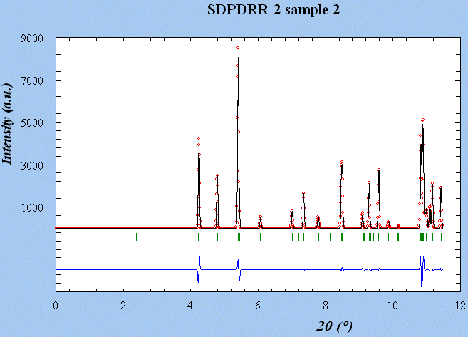
SDPDRR2 Sample 2 (sample2.dat) : monoclinic - > 6 minutes
Start : 17-Oct-2002     18 hour 35 min 36 Sec 
Rp        Vol           Ind        a              b             c       alpha      beta      gamma 
0.033   1760.121  22    19.9496   8.1937  11.2441  90.000 106.736  90.000 
    M(20) =    101.8119 
    F(20) =    588.4827     (  9.1853255E-04,           37) 

SDPDRR2 Sample 3 (sample3.dat) : cubic - 1 second
Rp        Vol           Ind        a              b             c       alpha      beta      gamma 
0.056   6735.840  24    18.8856  18.8856  18.8856  90.000  90.000  90.000 
    M(20) =    149.7873 
    F(20) =    512.6646     (  7.2244194E-04,           54) 

Test 1 - Cd3(OH)5(NO3) (test1.dat) - orthorhombic - 3 seconds
Rp        Vol           Ind        a              b             c       alpha      beta      gamma 
0.037    378.227   20    11.0279   3.4202  10.0277  90.000  90.000  90.000 
    M(20) =    126.0809 
    F(20) =    183.3493     (  3.7614279E-03,           29) 

Test2 (test2.dat) - tetragonal -  < 1 second
Rp        Vol           Ind        a              b             c       alpha      beta      gamma 
0.083   1186.855  25    11.1886  11.1886   9.4809  90.000  90.000  90.000 
    M(20) =    32.65442 
    F(20) =    58.72479     (  9.4603244E-03,           36) 

Test3 (test3.dat) - orthorhombic - 5 seconds
Rp        Vol           Ind        a              b             c       alpha      beta      gamma 
0.101   1154.716  25   11.3318   9.2362  11.0328  90.000  90.000  90.000 
    M(20) =    17.36584 
    F(20) =    29.50007     (  1.0593196E-02,           64) 

Test 4 : monoclinic  - less than 1 minute
Rp        Vol           Ind        a              b             c       alpha      beta      gamma 
0.077    684.950   25    6.2461  12.4695   9.1917  90.000 106.911  90.000 
    M(20) =    52.42331 
    F(20) =    110.0724     (  6.4892345E-03,           28) 

Test 5: (NH4)2S2O3 - monoclinic - 16 seconds
Rp        Vol           Ind        a              b             c       alpha      beta      gamma 
0.094    582.592   25    8.8043   6.4951  10.2231  90.000  94.757  90.000 
    M(20) =    33.04150 
    F(20) =    59.24461     (  7.1826265E-03,           47) 

Test 6 : triclinic - small cell - < 2 minutes
Rp        Vol           Ind        a              b             c       alpha      beta      gamma 
0.079    182.342   25     7.6256   5.5093   5.1169  89.828  74.979  62.441 
    M(20) =    37.16255 
    F(20) =    53.50393     (  1.2460144E-02,           30) 

Test7 - cubic ??? - < 1 second
Rp        Vol           Ind        a              b             c       alpha      beta      gamma 
0.110  13743.956 23    23.9536  23.9536  23.9536  90.000  90.000  90.000 
    M(20) =    6.623881 
    F(20) =    14.28700     (  1.7071631E-02,           82) 

Test 8 - monoclinic - < 2 minutes
Rp        Vol           Ind        a              b             c       alpha      beta      gamma 
0.098    149.517   20     5.0750   5.8569   5.0319  90.000  91.444  90.000 
    M(20) =    50.94925 
    F(20) =    54.74235     (  1.0148551E-02,           36) 

Test 9 - triclinic -  < 1 minute
Rp        Vol           Ind        a              b             c       alpha      beta      gamma 
0.069    984.080   20    7.0828  18.8631   8.7848 117.123  94.043  71.092 
    M(20) =    52.09227 
    F(20) =    135.3708     (  5.2765133E-03,           28) 

Y2O3 - cubic - < 1 second
Rp        Vol           Ind        a              b             c       alpha      beta      gamma 
0.073   1190.426  19   10.5983  10.5983  10.5983  90.000  90.000  90.000 
    M(20) =    136.5140 
    F(20) =    96.67932     (  3.9031976E-03,           53) 

See also the nameb.* files which are corresponding to the Black Box mode. 
See also the mixture1 and mixture2 files corresponding to the Two Phases mode. 

In mixture1.imp (2 cubic phases), the correct couple of solutions appears in 15th position : 

Rp2    Vol    Ind Nsol    a        b         c      alpha  beta  gamma
0.113 1078.288  29  7  10.2544  10.2544  10.2544  90.000  90.000  90.000
0.165 1190.411  14  7  10.5982  10.5982  10.5982  90.000  90.000  90.000

 Rp2    Vol    Ind Nsol    a        b         c      alpha  beta  gamma
0.259 1188.120  30 13  11.1880  11.1880   9.4919  90.000  90.000  90.000
0.106  378.244  15  4  10.0276   3.4206  11.0274  90.000  90.000  90.000

In 15-20 years, computers will be 2¹⁰ to 2¹³ faster (x1000 to x8000 faster), at least, probably. Even grid search in triclinic will be manageable. 
 

Parallel computing is clearly the best way now :
Dual core were available in 2005-6.
Quad core by the end of 2006, beginning of 2007.
80-core is announced for 2010-12...

I have done a lot already, wasting randomly considerable time ;-)... 

Parallelizing the grid-search mode is not yet done.

New bugs are occuring erraticaly in the parallelized version... Displaying sometimes NaN, infinit, etc instead of usually nice numbers... This is very probably due to incorrect assignation of some variables (shared or privates) in the Open MP directives. If you are an expert in parallelizing Fortran codes with Open MP directives, please help ;-).